With previous experience of improvement projects from over 25 companies, Elevantas offers three specialized consulting models perfect for companies looking to get started or gain an external perspective, our structured approach ensures minimal disruption and clear, actionable results
S&OPImplementation
Helps establish a robust process to balance supply and demand.
1. SupplyStrategy
ModelDefinition. (Make to Stock, Make to Order, Assemble to Order)
2. Technological Families
Divided products based on manufacturing process similarities
3. Data Structure
Define data architecture (data sourcing, modelling and visualization). Collect essential data
4. Demand Planning
Define demand forecasting, unconstrained demand definition and sourcing
5. Capacity Planning
Define Available capacity, collecting missing info and structure capacity check routine
6. Pre-S&OP Meeting
Discuss and evaluate solutions to balance supply and demand
7. S&OP session
Close the S&OP cycle by formalizing demand and production plan with executive team
Lean basics Implementation
Focused on identifying and eliminating waste in value creation processes.
1. Business Modeling
Understand how value is generated, revenue and cost structure
2. Lean principles
Training on lean principles (5 principles, waste attack, kaizen)
3.Value Stream Mapping AS-IS
Map the current flow of material and information. Define Throughput and Lead Time
4. 5S Audit
Go on the shopfloor and launch activities to implement order
5. Waste Detection
Together with VSM is one of the tool to identify projects to attack losses
6. Waste Attack and Flow Creation
Launch quick wins to improve performances
7.Value Stream Mapping TO-BE
Define the future state of operations and projects to close the GAP
Diagnostic Analysis
A holistic evaluation of operations with a scoring system.
1. Business Modeling
Understand how value is generated, revenue and cost structure
2. Value Creation Mapping
Process Mapping: Order to Pay, Manufacturing, Bid to Cash
3. KPIs and Performance Data Analysis.
Analysis of past performance and Business Intelligence
4. Shopfloor Visit
Go on the shopfloor to analyze daily operations
5.Interviews
Talk with first line managers to define current state and criticalities
6. Improvement plan proposal
All the analysis and recommendation are formatted into a plan
7.Audit Score
Evaluate the current situation and define the GAP
Walk the talk: how do we address an S&OP project
What a better way than show a real example on how we operate? Something that we can show without any disclosure agreement as it is based on public data: WallMart past sales. Here how we tackle S&OP at Elevantas in six simplified steps.
1: Hands-on no surprises Approach
Our method is based on making complex things simple. We achieved that through our pre-established routes and templates
Predefined working routes
Already defined timelines (6 months for basic implementation)
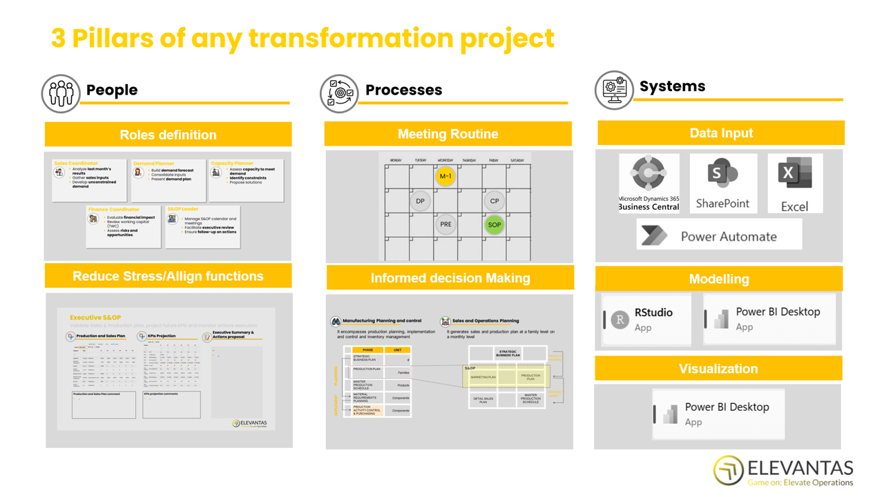
Holistic approach: People, Process and Systems
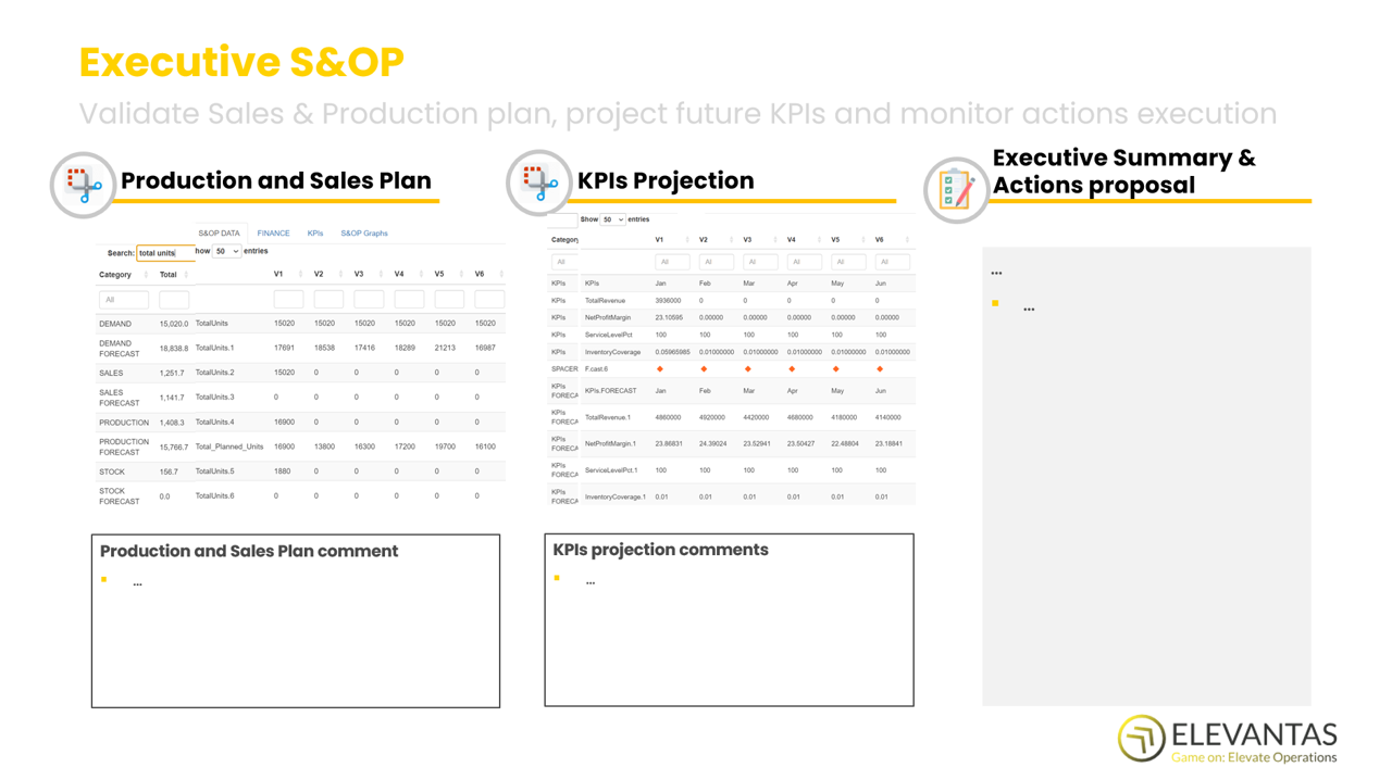
Start with the end in mind: Templates to clarify roles and meeting structures
S&OP Project phases
Project fundamentals
Example of template for S&OP meeting
Predefined working routes
Already defined timelines (6 months for basic implementation)
Holistic approach: People, Process and Systems
Start with the end in mind: Templates to clarify roles and meeting structures
S&OP Project phases
Project fundamentals
Example of template for S&OP meeting
2: Our method in practice – S&OP at WallMart example
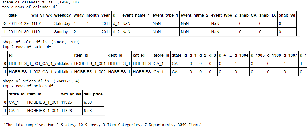
By using historical Walmart sales data we demonstrate a practical Sales and Operations Planning (S&OP) approach in a Make-to-Stock environment. By leveraging real-world data, we can showcase how demand forecasting and inventory planning can be optimized for large-scale retail operations.
Make-to-Stock: Demand is forecasted to drive inventory replenishment.
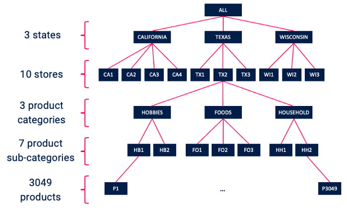
Items: 3,049 unique products (SKUs) included in the analysis.
Number of Stores: 10 Walmart stores across three U.S. states (CA, TX, WI).
Time Span: Daily sales data covering over five years.
Additional Data: Includes historical pricing, promotional events, and calendar information for enhanced forecasting accuracy.
Data structure
How the 3 starting files looks like
Data set from WallMart M5 forecasting challenge
Make-to-Stock: Demand is forecasted to drive inventory replenishment.
Items: 3,049 unique products (SKUs) included in the analysis.
Number of Stores: 10 Walmart stores across three U.S. states (CA, TX, WI).
Time Span: Daily sales data covering over five years.
Additional Data: Includes historical pricing, promotional events, and calendar information for enhanced forecasting accuracy.
Data structure
How the 3 starting files looks like
We are talking about Wallmart
3: Data understanding and modelling
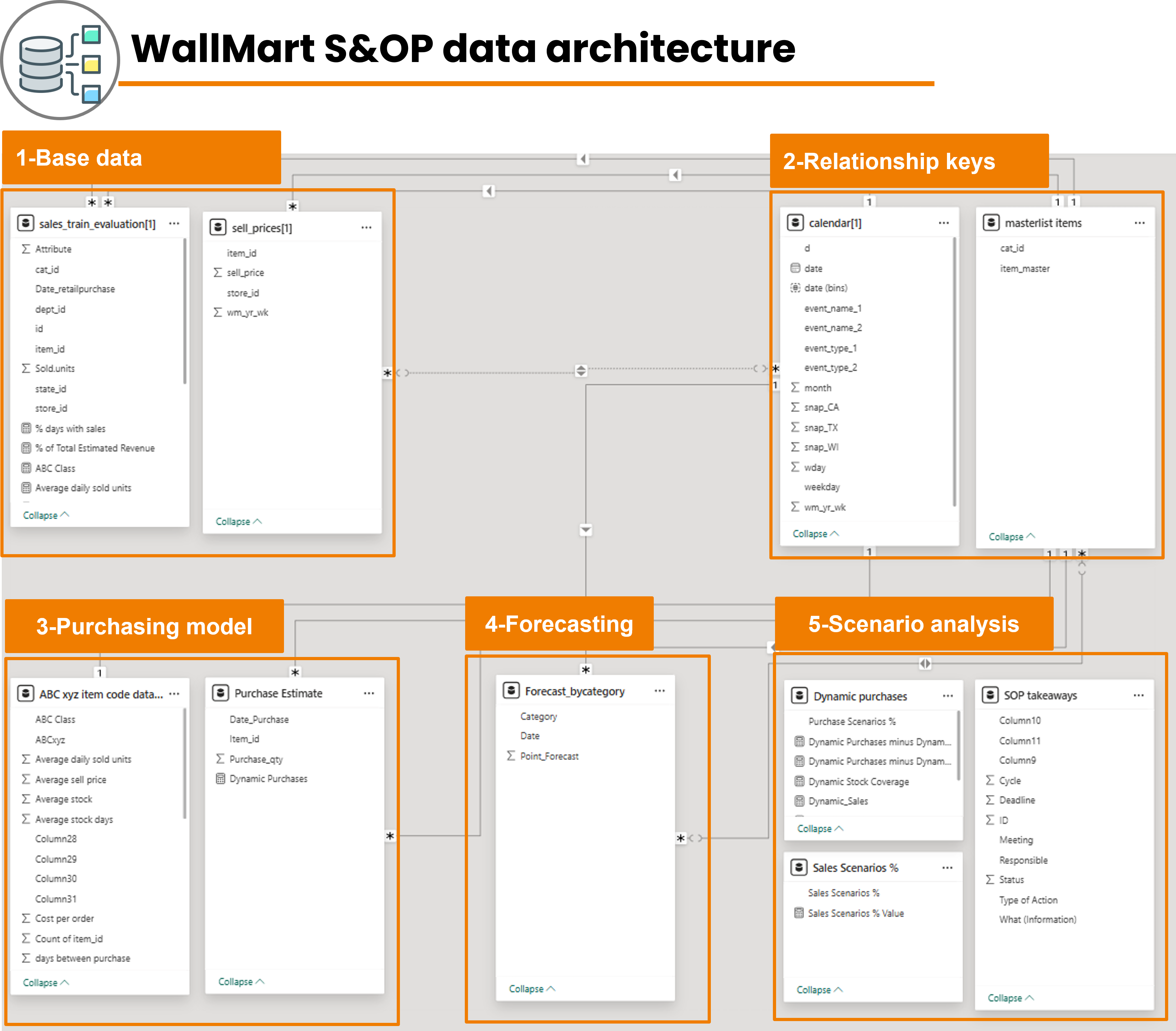
The original data are modelled into a data architecture system that supports S&OP. Through relationship keys the original sales table is connected to the purchasing model block, the forecasting block and the what-if scenario analysis block. Data interact to provide the necessary information taking advantage of technology.
Data Architecture: 5 Blocks interacting with each other to create a single database
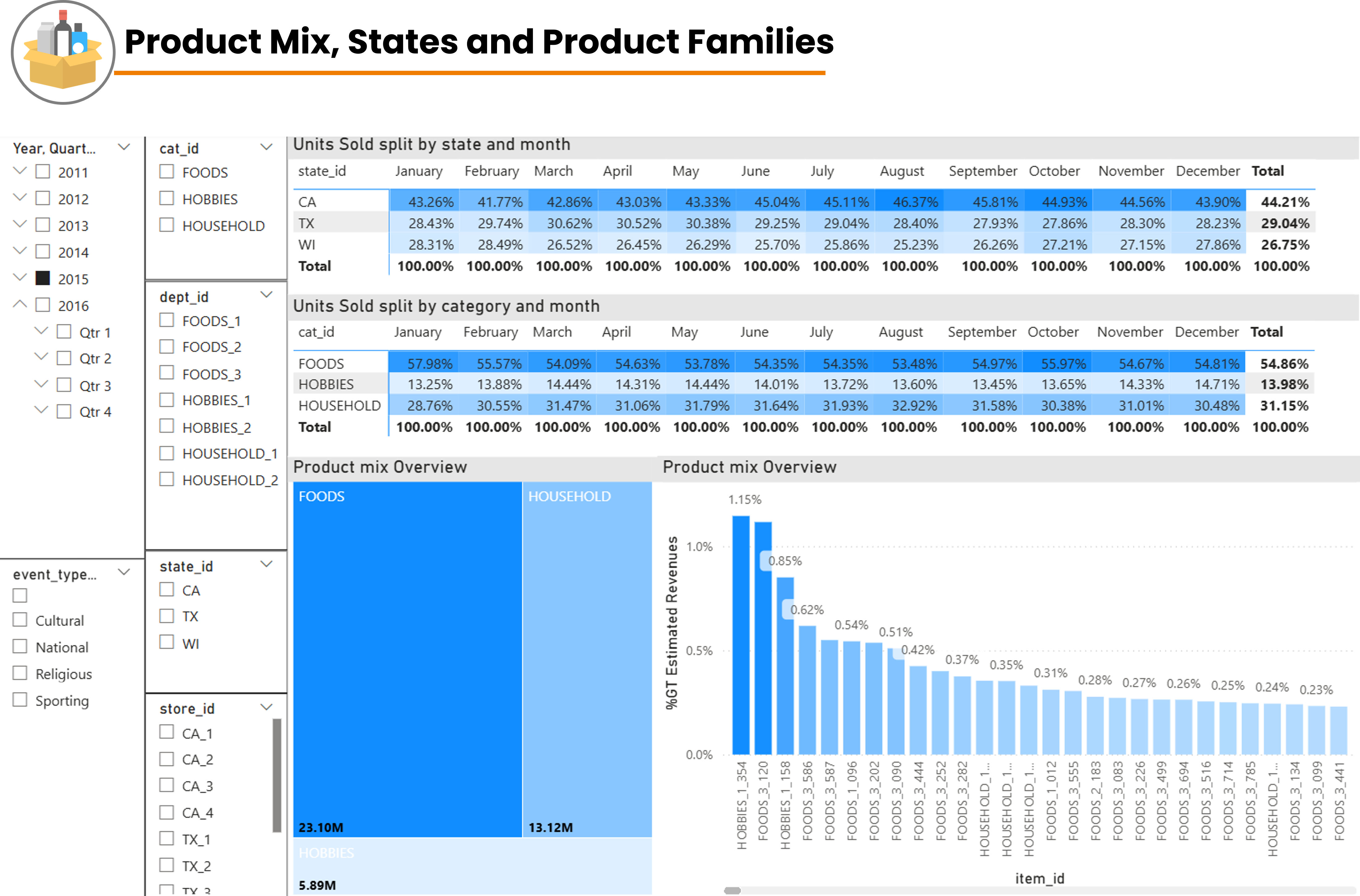
Sales Outlook: In 2025 the 3049 items sold around the 10 stores generated a volume of 13,8Mln units
Product Mix: Food category accounts for 54% of Sales. Top 20 codes account for 10% of Sales
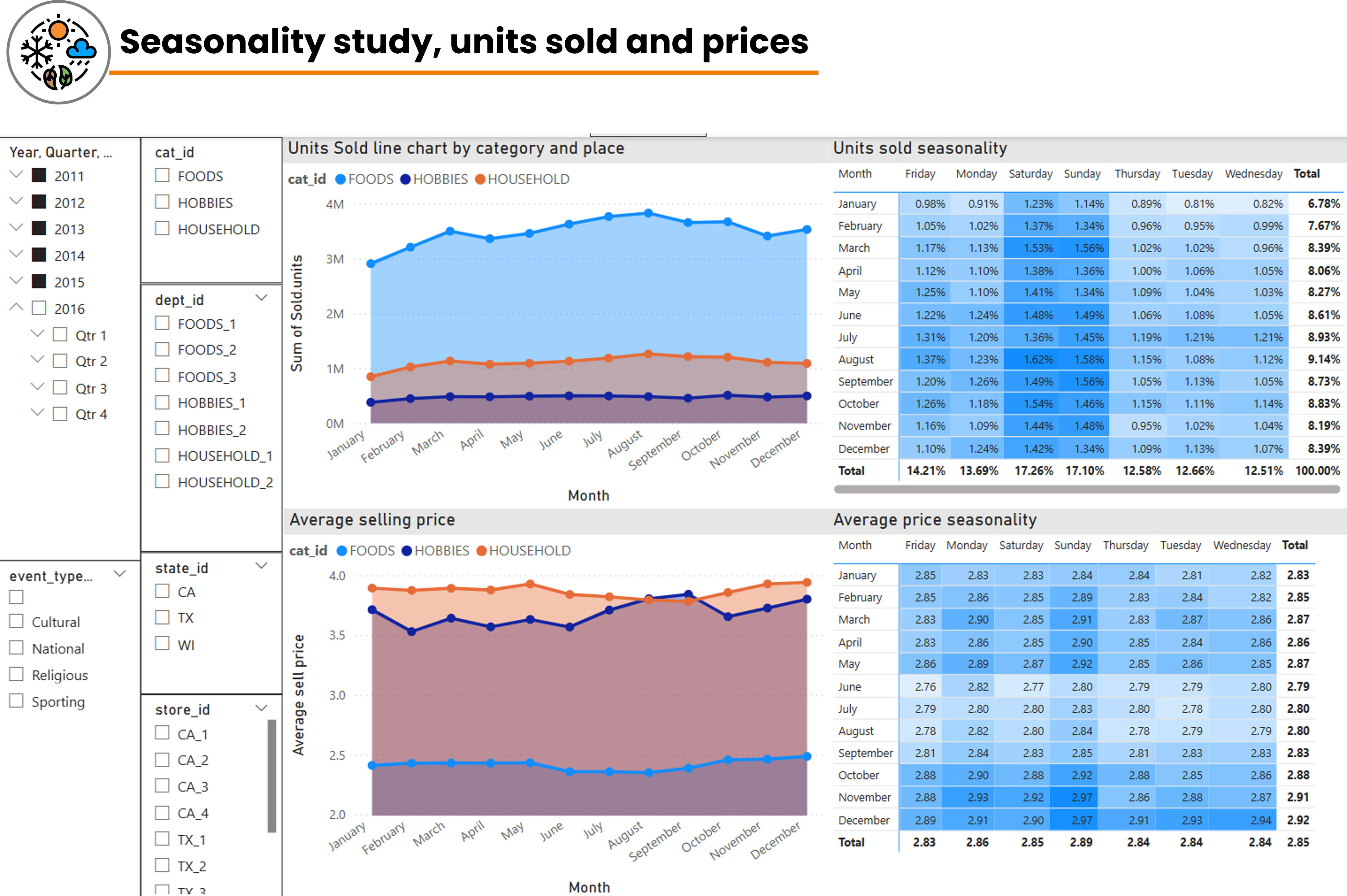
Seasonality: Strong weekly seasonality with weekends strong on sales. Summer shows higher sales for FOODS category alongside a reduction in average price
Data Architecture
Sales Outlook
Product Mix
Seasonality
Data Architecture: 5 Blocks interacting with each other to create a single database
Sales Outlook: In 2025 the 3049 items sold around the 10 stores generated a volume of 13,8Mln units
Product Mix: Food category accounts for 54% of Sales. Top 20 codes account for 10% of Sales
Seasonality: Strong weekly seasonality with weekends strong on sales. Summer shows higher sales for FOODS category alongside a reduction in average price
Data Architecture
Sales Outlook
Product Mix
Seasonality
4: Demand Forecasting
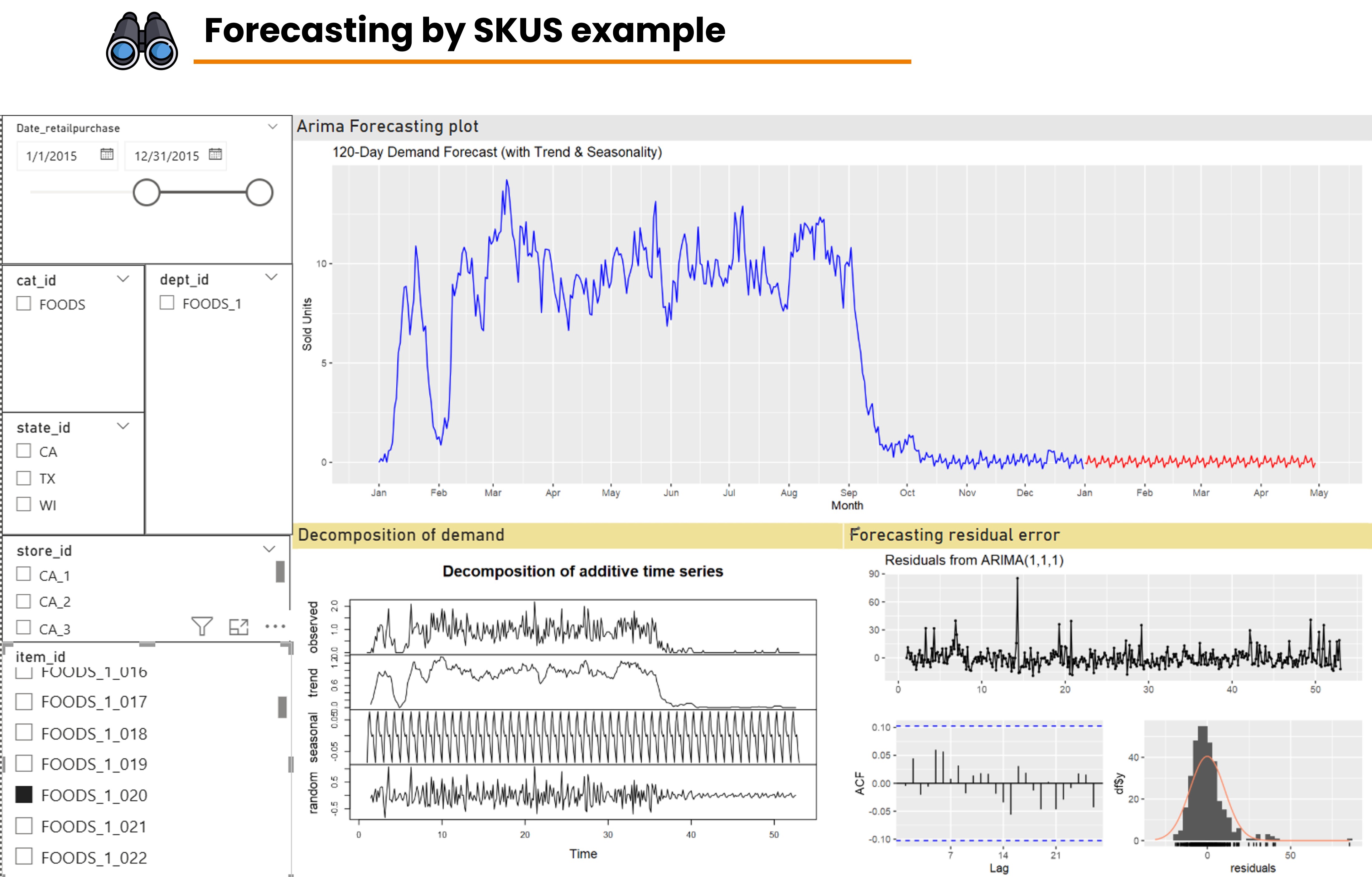
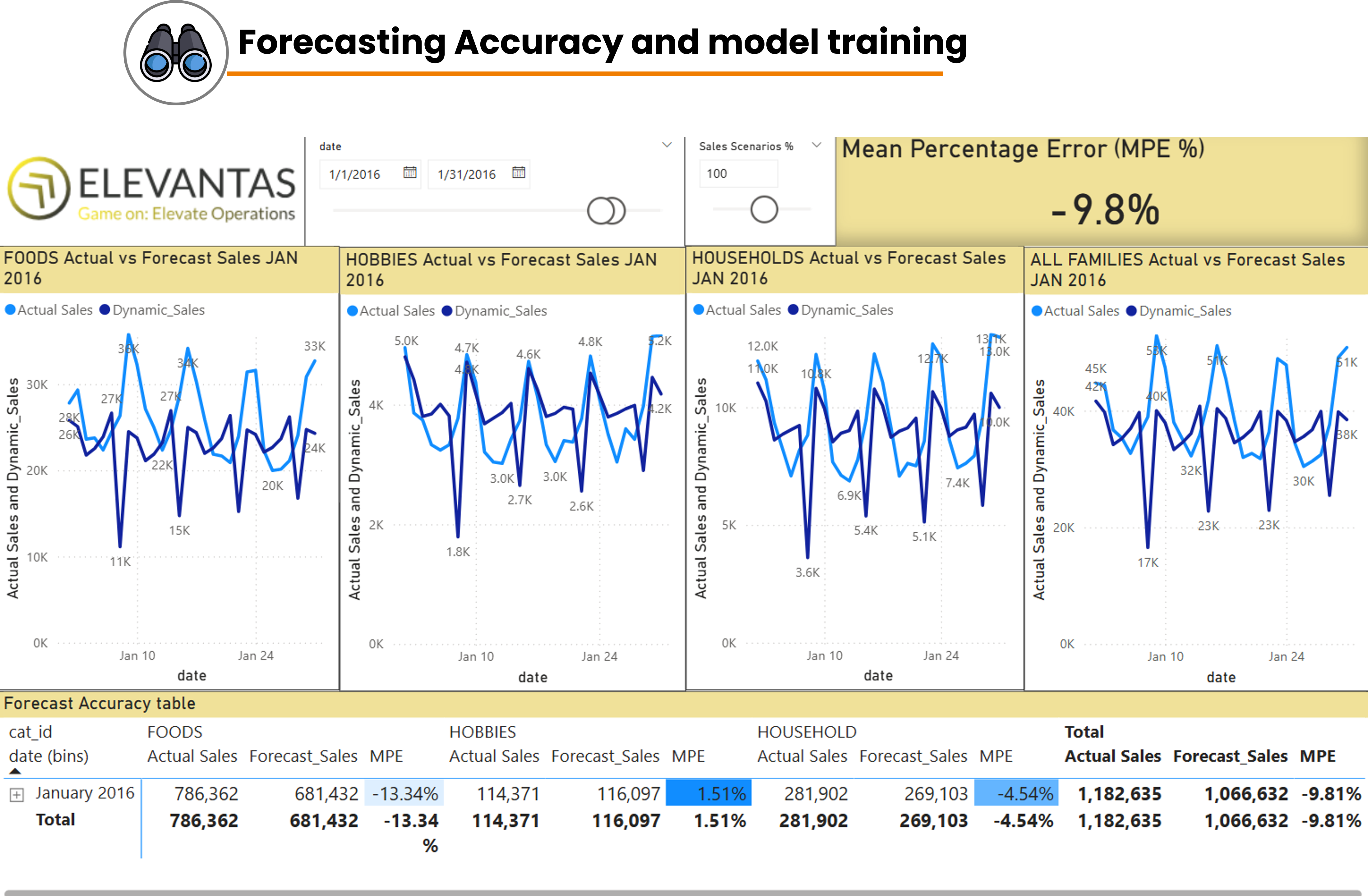
Dividing different group of products into forecasting categories is important for effective forecasting. we both developed an SKU and family level algorithm (based on ARIMA logic but with a twist to include seasonality and trend). By training the model with the real month data we achieved a MPE (forecasting mean percentage error) of 9,8%. At Elevantas we believe forecasting is a tool and not the end so we recommend focusing on the management part of the S&OP and stick to simple forecasting techniques
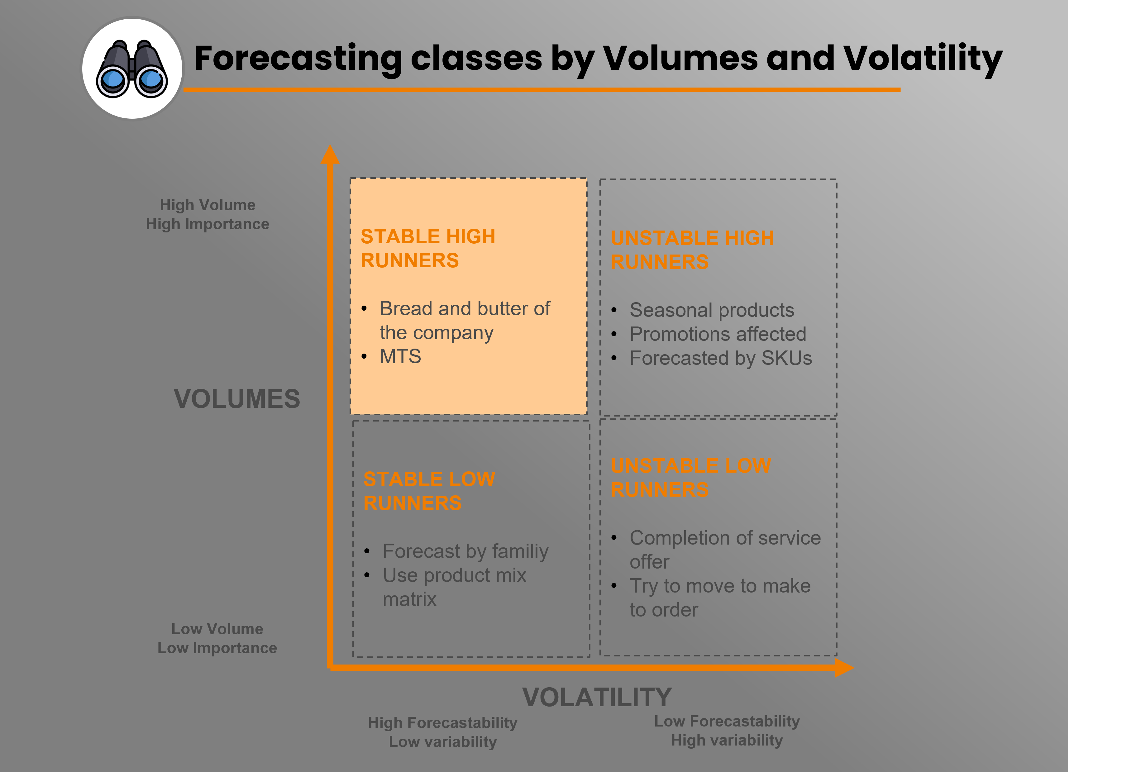
Volumes and Variability matters: By the matrix volumes/variability different forecasting families emerge.
Forecast by families: low runners and low volatility high runners are suitable for group forecasting
Forecast by SKUS: items with high volatility as influenced by seasonality, new launches or dismissal and promotions
Forecasting techniques: While keeping forecasting as simple as possible few categories might be needed:
Time series forecasting: for stable products (ARIMA technique is an example)
Linear modelling forecasting: for items that highly depend on other variables (eg price or promotions)
Qualitative forecasting: for products where very little past information is present
Forecasting Accuracy: Forecasting is an ever ending process that iterates from its error to keep improving and serving management team to take better decision. MPE (mean percentage error) is a good place from where to start. We noticed the FOODS category was under-forecasted mostly due at 3 daily spikes. The model caught well the trend for weekly seasonality
Forecasting Matrix by volumes and variability
Forecasting at SKU level
Forecasting accuracy and monthly aggreagate view
5: Capacity Planning (Purchasing or Production)
In our case a purchasing model has been defined so to project future purchases to be able to define it they meet capacity, trade working capital constraints and inventory coverage levels
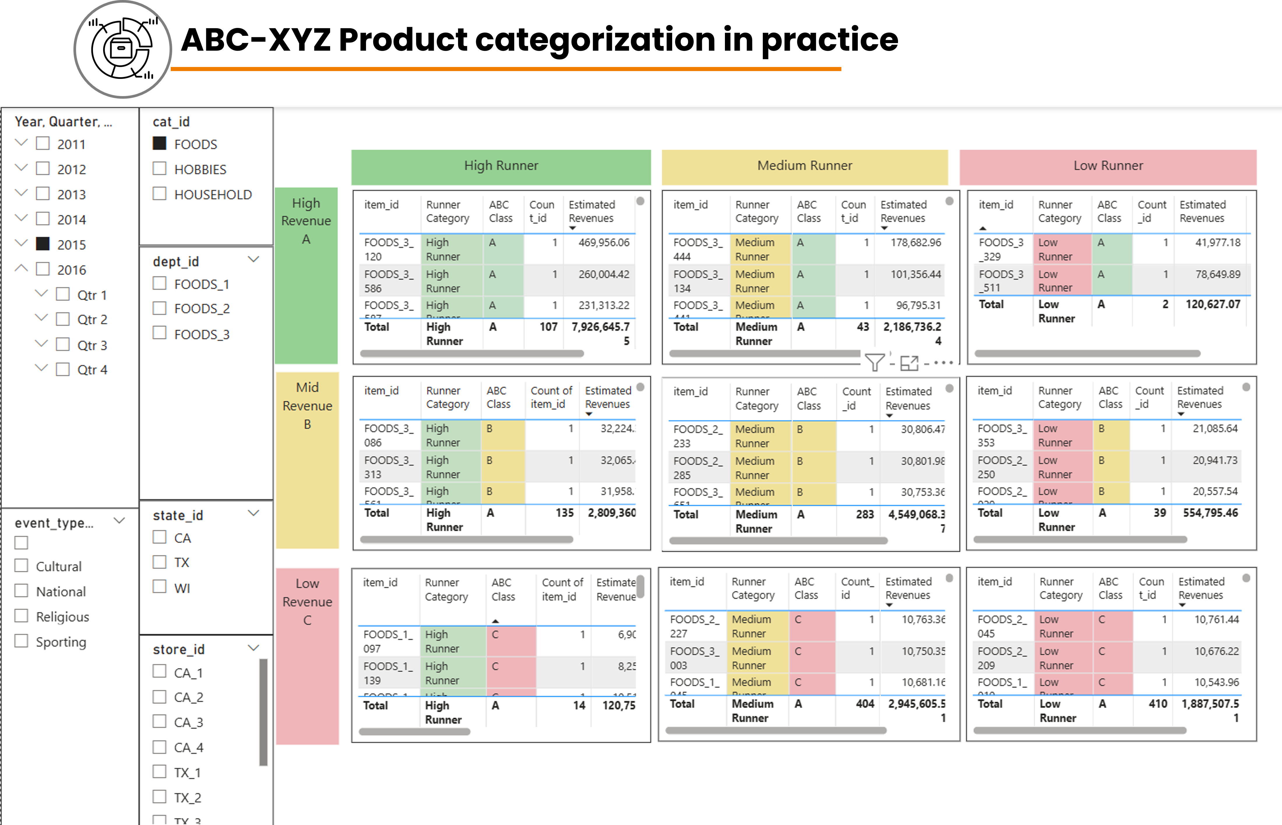
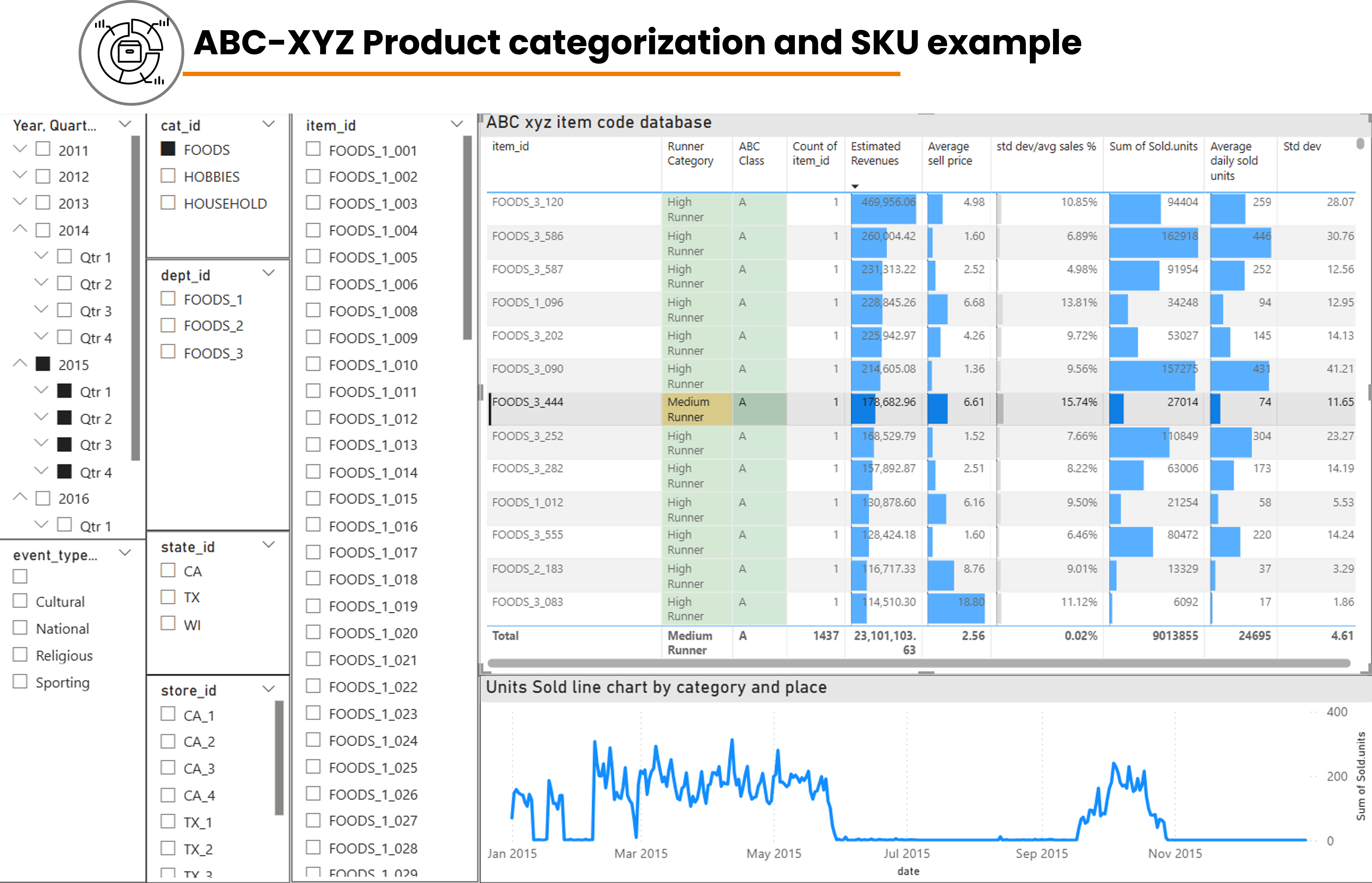
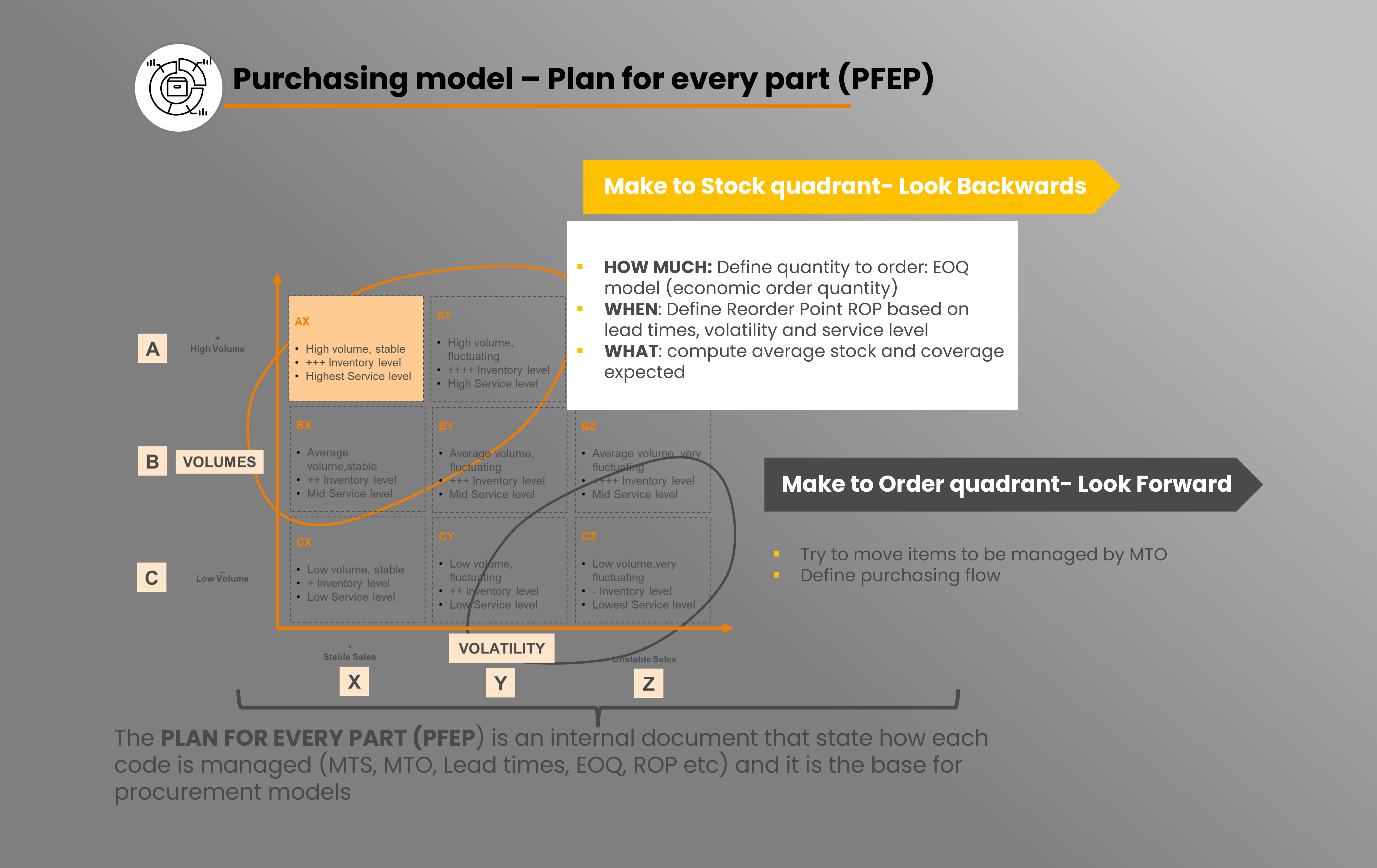
ABC-xyz Volume Frequency Matrix: the 3049 items got categorized by their consumption volumes (A,B,C) and their consumption volatility and frequency (measured by consumption standard deviation). this way 9 categories are generated each one with different»:
Forecast by families: low runners and low volatility high runners are suitable for group forecasting
Forecast by SKUS: items with high volatility as influenced by seasonality, new launches or dismissal and promotions
Plan For Every Part: Starting from the ABC xyz management decisions have to be taken on how to treat each item (MTS, MTO). For each item the following has to be defined:
How much to order: Economic Order Quantity EOQ
When to order: Reorder point ROP
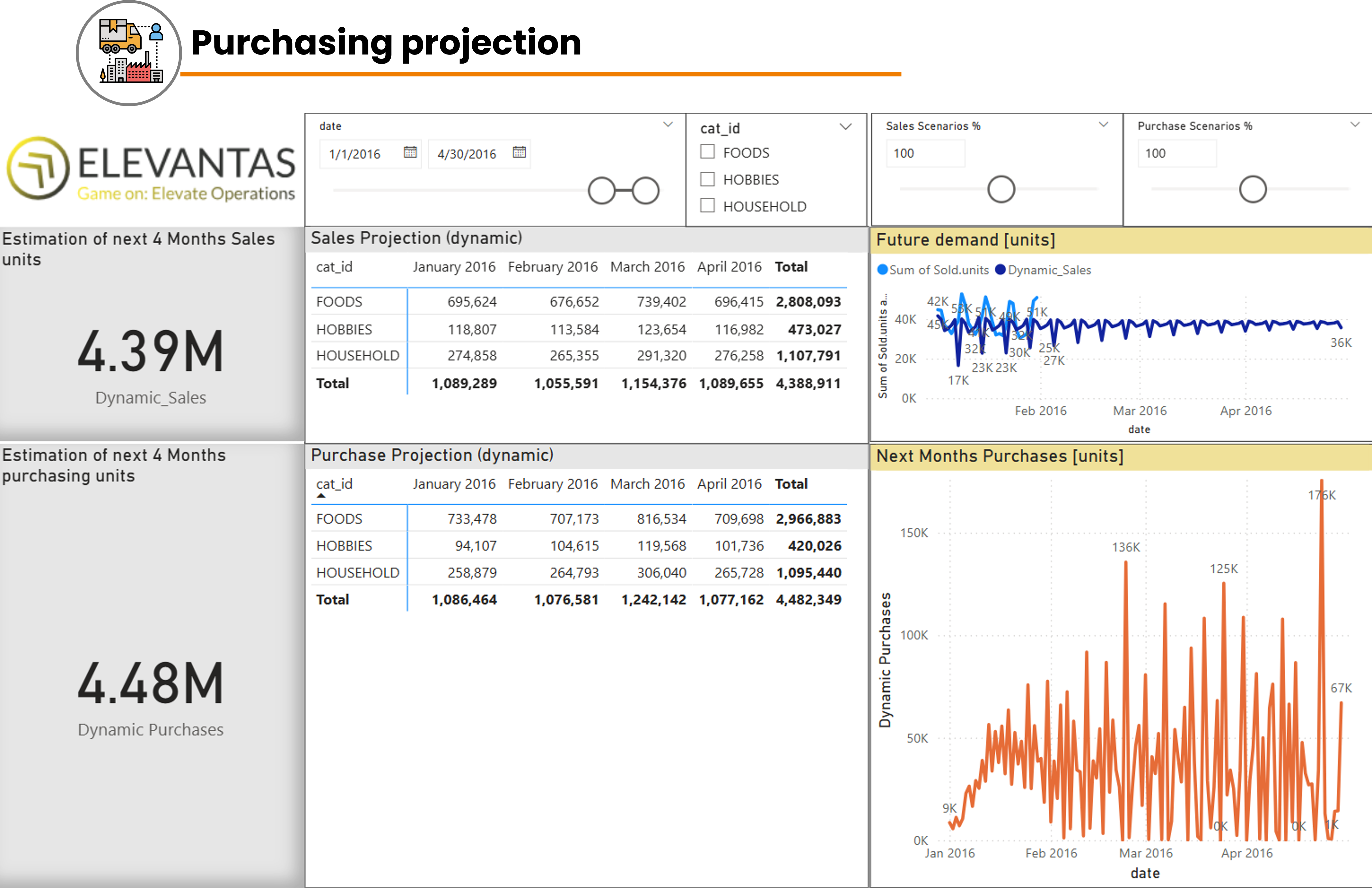
Purchase Projection: Now, once PFEP is formulated we can check the projection of future purchases. In our case, for January a 4,48 Mln units purchasing projection is estimated with Forecast sales of 4,39Mln meaning the purchasing model looks solid
ABC xyz Matrix for inventory management
ABC xyz matrix for WallMart case
ABC xyz matrix for WallMart case SKU view
Developing a Plan For Every Part
Projecting future Purchasing for January 2016
ABC-xyz Volume Frequency Matrix: the 3049 items got categorized by their consumption volumes (A,B,C) and their consumption volatility and frequency (measured by consumption standard deviation). this way 9 categories are generated each one with different»:
Forecast by families: low runners and low volatility high runners are suitable for group forecasting
Forecast by SKUS: items with high volatility as influenced by seasonality, new launches or dismissal and promotions
Plan For Every Part: Starting from the ABC xyz management decisions have to be taken on how to treat each item (MTS, MTO). For each item the following has to be defined:
How much to order: Economic Order Quantity EOQ
When to order: Reorder point ROP
Purchase Projection: Now, once PFEP is formulated we can check the projection of future purchases. In our case, for January a 4,48 Mln units purchasing projection is estimated with Forecast sales of 4,39Mln meaning the purchasing model looks solid
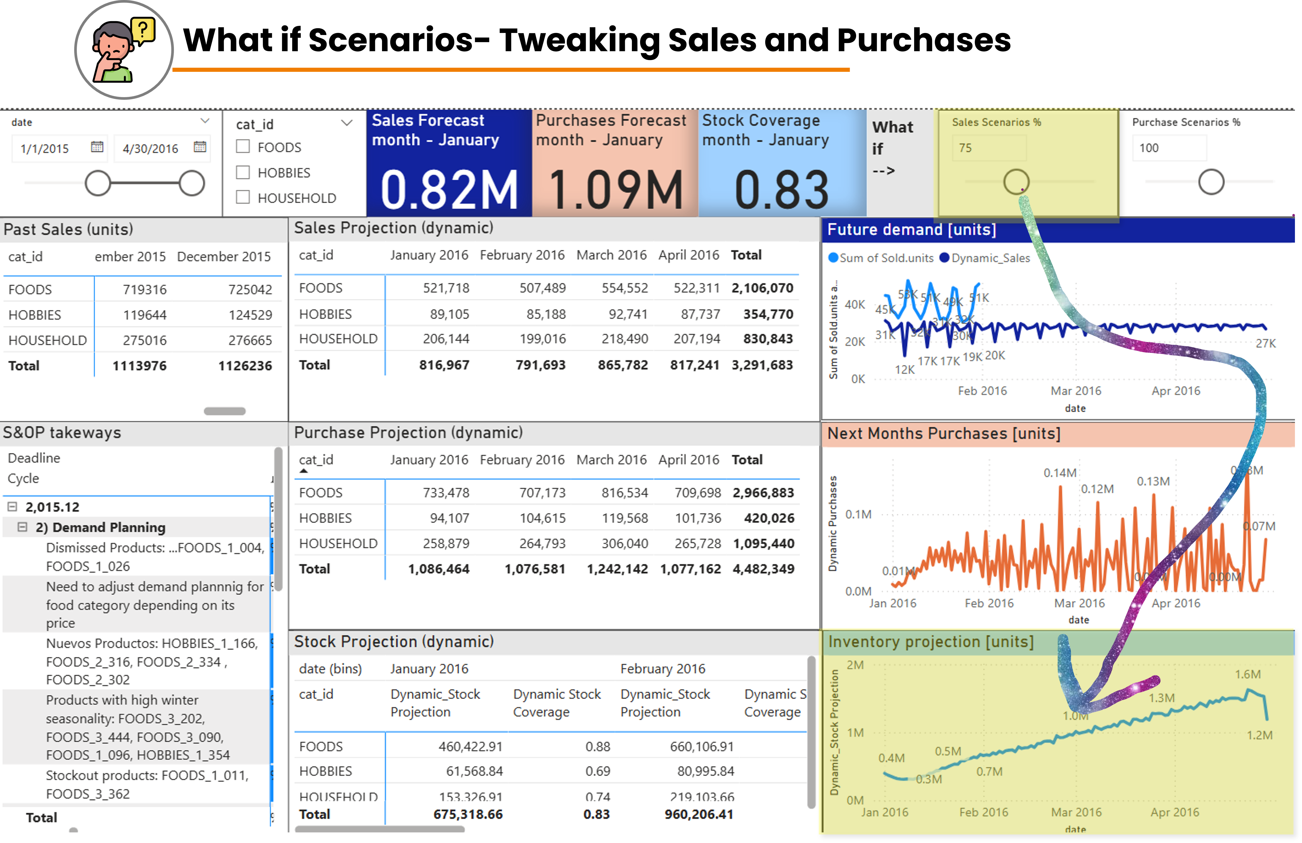
All the previous work finalizes in the S&OP cycle which is a set of meetings culminating in the Executive S&OP, where all the team agrees over data, decisions and set scenarios to see what would happen in case hypothesis are not met (we simulate a scenario with 75% of estimated sales and see the impact on stock)
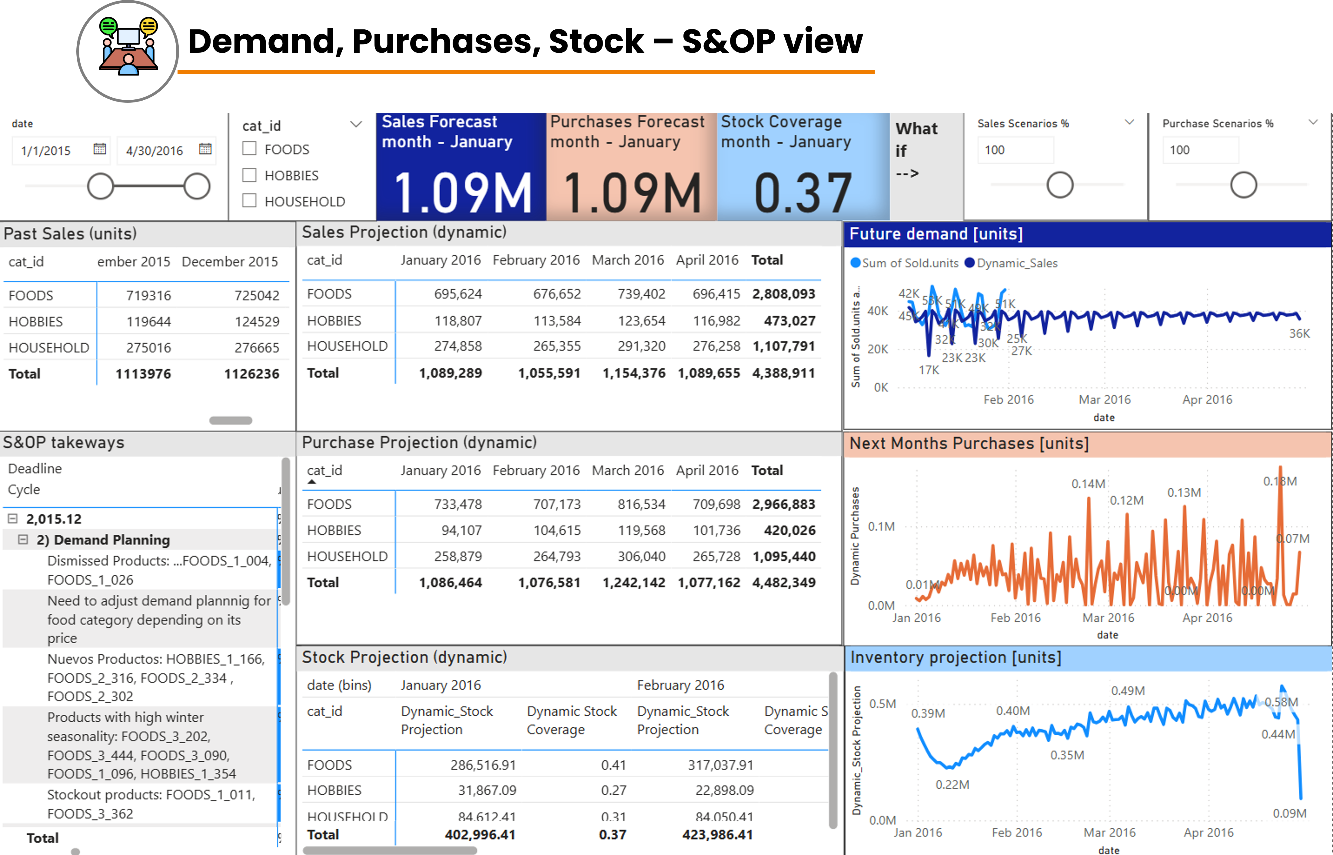
Inventory Levels output based on Sales and Purchase projection: the S&OP view encompasses key unique and reliable information for the entire team (January example)
1,09 Mln uds Sales
1,09 Mln uds Purchases
0,37 months Inventory coverage
S&OP routine takeaways: All key information and decisions taken during S&OP cycle are written in takeaways minutes:
under-forecasting of FOODS category
New items and promotions
Dismissing items
Finance implication of current stock coverage
What if Scenario analysis: during the S&OP we can test multiple scenario by seeing the impact of different % of sales or purchases over the company performance. By setting Sales at 75% we obtained
0,82 Mln uds Sales
1,09 Mln uds Purchases
0,83 months Inventory coverage.
S&OP January complete view
S&OP scenario anysis with 75% of estimated Sales
Inventory Levels output based on Sales and Purchase projection: the S&OP view encompasses key unique and reliable information for the entire team (January example)
1,09 Mln uds Sales
1,09 Mln uds Purchases
0,37 months Inventory coverage
S&OP routine takeaways: All key information and decisions taken during S&OP cycle are written in takeaways minutes:
under-forecasting of FOODS category
New items and promotions
Dismissing items
Finance implication of current stock coverage
What if Scenario analysis: during the S&OP we can test multiple scenario by seeing the impact of different % of sales or purchases over the company performance. By setting Sales at 75% we obtained